This text was posted on Demotrends by Maarten Bijlsma on September 1, 2015. The original can be found here.

The fields of epidemiology and demography are closely aligned. Even demographers interested in fertility or migration, not just mortality, can learn a great deal from epidemiology. As a recent study has argued, epidemiology is currently undergoing a methodological revolution, and this is likely to affect demography as well. The epidemiological revolution is, in fact, a causal inference revolution. In this post, I describe G-computation, a technique which is used by scientists employing a causal inference approach. G-computation allows users to infer population-level effects from individual-level effect estimates, and can therefore be of great value to demographers.

Inferring a population-level causal effect: counterfactuals

Imagine a situation where we wish to know the real effect of mosquito nets on preventing malaria infections. With the ‘real’ (or causal) effect here is meant the difference in the risk that a random individual from our study population would have if (s)he is given a mosquito net, versus if this same person had not received this net. Of course, we can never observe the same person getting the net and not getting it. The situation that we didn’t observe for an individual is called the counterfactual (as it is counter to the fact that was observed). So when applying counterfactual theory in statistics, we hope that we can find sizeable groups of people that share similar relevant characteristics, both with and without mosquito nets. If these conditions are fulfilled, we can estimate the risk of malaria infection within the different groups in the study population. Fortunately, the only characteristics that are relevant in this analysis are confounding variables. Confounding variables are variables that affect both the outcome of interest (i.e. getting a malaria infection) and the determinant of interest (i.e. having a mosquito net); if we do not control for them, they will distort our estimate of the effect mosquito netting on getting a malaria infection. All other variables, if not included in our estimation model, do not bias our estimate of the causal effect of the intervention, and so can be ignored.

(Non-)collapsibility

In this imagined scenario where we want to know the causal effect of mosquito nets on preventing malaria infections, let’s say that we have a large sample size randomly drawn from the study population, and we have information on presence of mosquito nets and confounders. We could then fit some regression model, perhaps a logistic regression model, with malaria infection as the outcome variable, and with presence of nets and the various confounders as covariates. Our model could be specified as follows

Where p_i is the probability of getting a malaria infection, X₂ is a binary variable indicating the presence or absence of mosquito nets, X₃ is a continuous variable representing socio-economic status, and X₄ is a continuous variable representing age. For the sake of the argument, let’s say that socio-economic status and age are the only confounders, because the principle works the same if there are more confounders. Since these two variables are the only confounders, the estimate that we get out of this model is an estimate of the causal effect. However, because logistic regression uses a logit link, the effect estimate is also a conditional estimate; it is conditional on the other covariates (the confounders) in the model. That means that (1) it is not a good estimate of the effect on malaria infection of giving everyone (or a large group) in the study population mosquito nets (AKA the population-level causal effect), and (2) the estimate is not comparable to effect estimates in models with a different set of covariates. This issue is also known as non-collapsibility, and holds for the parameters of interest estimated by a large variety of models, including the odds ratio and the hazard ratio (but not linear regression). Fortunately, quite a few researchers are aware that conditional effect estimates are not necessarily equal to population-level effect estimates. However, point (2) is unfortunately still ignored by researchers, as even in good journals models with slightly different sets of covariates are compared to determine mediation or confounding, when the outcomes of those models are non-collapsible. Furthermore, certainly in demography, few are aware of how to solve either issue. G-computation to the rescue!

G-computation: direct standardization

In demography, when we want to compare mortality or fertility rates between countries, we commonly apply direct standardization. We might, for example, weight age-specific rates by the proportionate size of each respective age category, and then sum them to get an age-standardized estimate. G-computation is also a method of direct standardization, and therefore works according to the same theoretical principle. However, since the nature of the data (individual-level versus aggregate level) is different, the implementation of the method is also different.

If the sample that we work with is a random sample from our population of interest, the implementation is actually quite simple. First, using the regression model which controls for confounders, we can calculate the risk of malaria infection for each individual in our dataset as if they had access to mosquito netting. This is done by setting the mosquito netting variables to 1 for all individuals, while letting the other variables take on the values that were actually observed. For example, if our earlier specified logistic regression model had as its estimates β₁ = 0.2, β₂ = -0.9, β₃ = -0.1, β₄ = -0.03, then for a person with socio-economic status of 0.6 and an age of 20, the logit probability of malaria infection would be

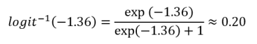
Applying the inverse logit function this person therefore has an estimated probability of malaria infection of

In a second step, we now use the regression model which controls for confounders to calculate for each individual in our dataset the risk of malaria infection as if they had not had access to mosquito netting. So for our example person, then logit probability would then be

the probability of malaria infection for this individual is then

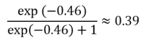
Which means that, for this individual, we estimate that the causal effect of having a mosquito net is 0.39-0.20 = 0.19 lower probability of getting a malaria infection. Note that, if we had used someone with a different age, but otherwise the same covariates, the difference in risk would have been different, even though there are no interaction effects in the model. Hence the need to calculate this risk for all individuals in the dataset separately. In other words, we estimate the counterfactual outcomes for each individual in our dataset! Once the probability of malaria infection has been calculated for each individual, both with and without having a mosquito net, we can calculate the population-level effects. This is done by taking the average probability of malaria infection when everyone has malaria nets, and the average probability in the group where no one has nets, and subtracting these averages from one another. This calculated value represents the difference in the probability of getting malaria infection if we gave everyone in the study population mosquito netting, versus if we made sure nobody in the study population had mosquito netting. Standard errors for our population-averaged estimate can be derived through bootstrapping.

When should we use G-computation?

As indicated, the technique is great if we want to get population-averaged estimates, which here I showed using the situation of everyone getting mosquito netting versus nobody getting mosquito netting. However, if desired, we can also simulate other scenarios; for example, we can compare the situation of 25% of the population having mosquito nets versus 75% having mosquito nets. Or we can investigate the influence of two interventions at the same time (possibly with a mixed distribution); e.g. some percentage of the population getting mosquito netting and education on malaria, another percentage getting only education, etc. The possible scenarios are limitless, as long as we have good empirical data.

The method is also very useful if we want to simply compare estimates from similar models with non-collapsible outcomes. When there are differences between the estimates of two similar models, the difference is not necessarily due to mediation or confounding, but may be due to non-collapsibility. So, if we want to make such a comparison between models, all we have to do is apply G-computation (using the individual-level data as explained above) to get population-averaged estimates from both models. We can then compare the two population-averaged estimates. We’re sure, then, that the difference between the two estimates is not due to non-collapsibility, but due to other sources (such as mediation). However, if the two models differ only by a few variables, but are otherwise the same, and the estimated coefficients of the additional variables are very small, the influence of non-collapsibility on an estimate is generally very small and G-computation would not be necessary.

Like any method, G-computation also has limits. For one, while G-computation can help with adjusting for confounding, it cannot protect against unmeasured confounding. Furthermore, the method is easiest to apply when we have taken a random sample from our study population. We need a random sample because the distribution of the covariates (confounders) in our sample should be representative of the distribution in the study population. Therefore, if instead we have some sort of oversample, application may still be possible but already becomes more troublesome. Finally, the method cannot be applied to models with time-varying variables. In the case of time-varying variables, we should instead use the parametric G-formula. The parametric G-formula is essentially G-computation on steroids, and perhaps the topic of a future post on Demotrends!