This text was posted on Demotrends by Maarten Bijlsma on September 4, 2013. The original can be found here.

Most researchers are familiar with the difference between bias and precision. However, not everyone knows that we can allow for a little bit of bias in order to get big gains in precision, and when it can be beneficial to do so.  In this post I detail the why and how.

A refresher on bias and precision

So what were bias and precision again? Being unbiased means, statistically, that our method of estimation is correct ‘on average’. Whenever we estimate something, the estimate that we would get based on a random sample is usually not exactly right. However, if we took infinitely more random samples and re-estimate for each of these samples, then the average of all of these estimate would equal the true value that we are trying to estimate. If this average of many estimates is not correct, then our estimator (this is we call our method of estimation) is biased. Having a precise estimator means that our estimates are usually close to the true value that we seek to estimate; so precision is the inverse of the variance of our estimator. If we really did take an infinite number of samples, we would find that an estimator has a distribution, see Figure 1 for example. The distribution of the red estimator shows that some of its estimates will be far away from the true value, but most are usually quite close to the true value. The figure also shows that the red estimator is generally better than the blue estimator (they are both unbiased, but estimator 2 has a smaller variance). But what about the purple estimator? It has a smaller variance than estimator 1 and 2, but it is not centered around the true population value; it is biased.

Figure 1: the distribution of three estimators (true value: 5). The purple estimator has the smallest variance but is biased (its mean is 5.2 whereas the means of the other two distributions are 5). These distributions were generated in R using 100.000 samples of n = 20 for each estimator.

The variance of estimators

It is well-known that using less precise scientific instruments for our measurements will increase variance in our data and (therefore) in our estimators. However, even if our research design and the actual sampling from the population are flawless, our method of estimation itself (the estimator) can still be a source of (increased) variance. Many applied researchers are not so familiar with the fact that many parameters (the things we want to estimate) can be estimated using different methods. For example, methods of finding good estimators are the method of maximum likelihood, the method of moments and the Bayesian approach. Of these, maximum likelihood will probably ring a bell: estimators constructed following this method are guaranteed to have the smallest possible variance out of all unbiased estimators and so are commonly used. If the estimator is indeed also unbiased, then we refer to this estimator as a minimum variance unbiased estimator (MVUE). Sometimes we still use a different estimation method simply because it is more convenient to do so. But how can one method of estimation have a higher variance than another? Let’s take outcomes with a Poisson distribution as an example. The Poisson distribution is governed by only one parameter; both the variance and the mean of data generated from a Poisson distribution are determined by this parameter. So we could take the mean of our data or the variance of our data as estimates of this parameter. Which is better? Well, the blue lined distribution in Figure 1 is an estimator based on the variance, and the red line is based on the mean: clearly both are unbiased but the mean-based one has a much smaller variance. For the Poisson distribution, taking the mean is in fact the MVUE. However, even if we are working with MVUE’s we can get very high variance. For example, a common source of very high estimator variance is multicollinearity; this occurs when we have a number of variables that are strongly tied together in their prediction of the response. This means we don’t know which of these variables is truly responsible for the change in the response variable and therefore we have a lot of uncertainty in our estimates.

A trivial example or: how to get the best possible precision by increasing bias

So how can we go about reducing variance by increasing bias? Well, it turns out there is a very simple way to reduce the variance of an estimator to 0. Namely, simply choose some constant (e.g. ‘14’): no matter what observed values are found in our random sample, we will always estimate 14 and hence our estimated values will not vary. Unless the true value of the thing that we are estimating happens to be 14, our estimator will be (extremely) biased.

Mean squared error

Clearly, the previous example shows that we are interested in more than just variance reduction; we want a good estimator. This is where the concept known as mean squared error (MSE) can help. Basically, MSE expresses how close, on average, an estimator is to the value that it needs to estimate. This may seem similar to the variance. However, as equation 1 shows below, it is actually more than that:

Equation 1. The Mean Squared Error (MSE).

Equation 1 shows us that the MSE is the average (roughly, this is what the E or expected value denotes) of the square of the distance between our estimates (denoted by W in the formula) and the true value in the population (denoted by theta) that we seek to estimate. This can be decomposed into the variance of our estimator (Var W in the formula) and the squared bias. So MSE nicely combines both things we want to take into consideration: bias and estimator variance!

Since the contribution of bias is always positive (because it is squared), that means that bias in the model will actually increase the MSE. So beware: just adding bias to a model without any further thought is not going to work, it will just make things worse. Methods that achieve variance reduction through the introduction of some bias can be seen as improvements when they don’t just increase the bias, but (by doing so) they also make the variance of the estimator much smaller (the Var(W) part in the formula). So we can only get an overall improvement if we can get the reduction in the variance of our estimator to outweigh the increase in squared bias.

A real example or: how to really get some precision improvements

Many methods have been developed which can increase precision by increasing bias (in a reasonable way), especially in the field of data mining. Here I will give one example that I personally consider to be quite brilliant: the Least Absolute Shrinkage and Selection Operator (LASSO). Roughly speaking, the LASSO is an adaptation of a method that virtually all scientists have used: Ordinary Least Squares (OLS) regression. In OLS regression, we try to find a line which minimizes the sum of squared distance between itself and our observations. Mathematically, this is described in the least squares ‘normal equations’ (see equation 2):

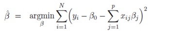
Equation 2. The Least Squares Normal Equation.

The basic idea of the LASSO is that we want to limit the range of our parameter estimates (here denoted with beta hat), because the greater that range, the greater the variance. As described above, when we have multicollinearity, our estimator can ‘blow up’ and potentially take very high values, which strongly increases variance. So one approach is to penalize values of our parameter estimates with a high magntitude (high positive or negative values), so that these will be estimated less by our model. This is basically what the LASSO does (see equation 3):

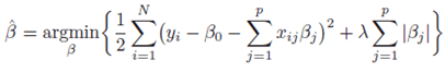
Equation 3. The Least Absolute Shrinkage and Selection Operator (LASSO).

Comparing equation 2 and 3, we see that a third term has been added. The lambda value we see in this model penalizes high parameter estimates; the higher lambda, the more we penalize high values and therefore the more we reduce variance. Next to reducing variance, a useful property of the LASSO is that, if we have a lot of variables and (therefore) high multicollinearity, the LASSO can set some parameter estimates to 0 entirely, thereby excluding unneccesary variables from our model. Unfortunately, penalizing high values also means that our estimates (and the distributions of our estimators, remember Figure 1) will tend more towards 0 (called shrinkage), thereby introducing bias in our estimation. Fortunately, often introducing just a tiny bit of bias can result in great gains in precision.

How all of this is helpful to quantitative researchers

What is the point of having greatly increased precision if, on average, our model is wrong (biased)? Well, while the model is wrong ‘on average’, it will still be more ‘more right’ most of the time if the MSE of the biased estimator is smaller than that of the unbiased estimator. Researchers usually have only one sample of data that they get to work with, so the argument of being wrong ‘on average’ is misleading. Effectively, we have only one shot at the truth and these methods make it more likely that our shot is as close to the truth as we can get it.